|
FB Mathematik und Informatik, Universität Bremen, 2800 Bremen,
FRG. Introduction Applying mathematics to problems in biology and medicine has a
long history dating, at least, to the work of Fibonacci in the thirteenth
century. In the twentieth century mathematical ideas have had a
profound impact on population biology, genetics, epidemiology, and
neurophysiology. However, in many ways, mathematical biology is
still in its infancy. In such fields as molecular biology, cell
biology, immunology, and certain branches of physiology, mathematics
is just beginning to be recognized as a useful tool [4]. Many exciting
applications of mathematics to the life sciences are today concerned
with nonlinear phenomena. Very often the relationship between variables
is not linear by its very nature but it has to be treated linearly
or by linear approximation because of the lack of mathematical tools
handling the nonlinearity directly. Consider, for example, the,
in the life sciences ubiquitous, phenomenon of growing ( or shrinking)
populations (human beings, animals, plants, bacteria, cells, etc.).
for carrying out the necessary mathematical analysis, a common idealization
then is to assume a constant rate of growth. This is in contrast
to the real dependence of the growth rate on the level of population,
due to population pressure like crowding, abounded environment,
food restrictions, etc. (see later sections for a more detailed
discussion). During the last two decades there has been great success
in developing new mathematical concepts and tools to cope with nonlinear
phenomena (see the references given at the end of this paper; for
applications in the life sciences, see especially [2, 4, 9, 11,
14, 17]). In particular, techniques were developed dealing with
the by now famous concepts of "chaos", "fractals", and "cellular
automaton" which have already entered many disciplines. However,
these new developments have also shown that it may be extremely
difficult to treat even the simplest kinds of nonlinearity analytically
in a rigorous manner. Hence, another idea may be useful, which also
arose in recent years and by which nonlinearities can be treated
analytically if they come with certain properties of positivity,
like positive and increasing levels of population. In contrast to
what is possible for discrete nonlinear dynamic systems in general,
the concept of positive dynamic systems also allows nonlinearities
to be treated analytically in higher dimensions, i.e., for many
variables. The aim of this contribution is only to offer a first
impression for those Who are not yet acquainted with the concepts
mentioned, but Who want to know roughly what they are about. I do
not proceed in a mathematical manner by giving definitions and theorems,
but discuss simple examples and illustrate the underlying ideas.
The interested reader Who wants to know more is referred to the
references given at the end of the paper. 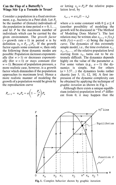
Nature presents itself rather differently from what mathematicians
usually depict in geometry. Leaves, clouds, coasts, lungs, mountains,
radiolaria, etc. are forms too complicated and too fantastic for
describing them in terms of Euclidean geometry [3, 10]. Nevertheless,
coping with these natural objects the scientist has to find some
way to measure those objects. The difficulties of measuring natural
forms in common terms have been pointed out by Benoit Mandelbrot
(1967) in an article entitled "How long is the coast of Britain?"
[cf. 10]. For measuring the true length one has to make the unit
of measurement E smaller and smaller and then to take the limit
case of all the lengths obtained. This does work even for curved
objects when they are smooth enough but it does not work for "fractional"
objects or fractals as are they named by Mandelbrot (for fractals
see [1,10,12,13,15,17]). Measuring the fractional coast of Britain
by making the unit of measurement smaller does increase the length
obtained to infinity, as is indicated in Fig. 2. In the article
mentioned, Mandelbrot refers to the British scientist Lewis fry
Richardson who had already, in 1961, analyzed measurements made
empirically for various coasts. Thereby he detected a magnitude
not for the length of the coast but for the "roughness" of the coast,
which was then called fractal dimension by Mandelbrot. More precisely,
the fractal dimension measures (in the above example) how much the
logarithm of the length L increases compared to an increase in the
logarithm of the inverse unit of measurement 1/h.. To put it in
a formula, the dependence of L on J:-' is given by the power law:
L=cE 1-d where d is the fractal dimension and c is some constant.
The fractal dimensions calculated for various coasts are strictly
greater than 1 (which is the dimension of a straight line) and strictly
smaller than 2 (which is the dimension of a plane). Today, the concepts
of a fractal and of a fractal dimension are used to measure surfaces
like those of lungs, blood vessel systems, or of materials in chemical
reactions. There are several possibilities in giving a precise definition
of a fractal. A fractal may be defined by the fact that the fractal
dimension does not coincide with the dimension in the usual sense
or it may also be defined by its self-similarity, (In fact, several
types of fractals have to be distinguished.) Another possibility
which, moreover, is very practical in constructing fractals using
the computer is the chaos game invented by Barnsley [1 ] which uses
a random process as in Fig. 3 a, b. Draw a (equilateral) triangle
in the plane with vertices 1, 2, 3 as shown in Fig. 3 a and mark
an arbitrary starting point in the plane. Throw a dice which is
assumed to show the numbers 1, 2, 3 only because any two opposite
faces of the dice are labeled with the same number. 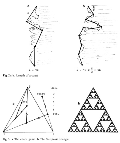 If the dice shows number n, then draw a line connecting the starting point with vertex 11 and obtain a new point by marking the middle point of it. Throw the dice again. If the dice shows number m, connect the new point obtained with vertex m by a line and mark on it the middle point as the new point. This process can be continued. What will be the figure formed by all the marked (middle) points? As it turns out, all these points arrange after a while on a classical fractal known for a long time as the Sierpinski triangle, shown in Fig. 3 b. The process described may also be considered as a dynamic system with the Sierpinski triangle as at tractor, that is, the motion of the system is finally attracted to the Sicrpinski triangle. Fractals appear as at tractors of nonlinear dynamic systems. (For the connection between fractals and dynamic systems as well as for an astonishing gallery of 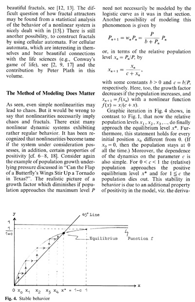
References 1. Barnsley M F (1988) Fractals everywhere. Acadcmic, Boston |